Here’s something I’ve been playing with:
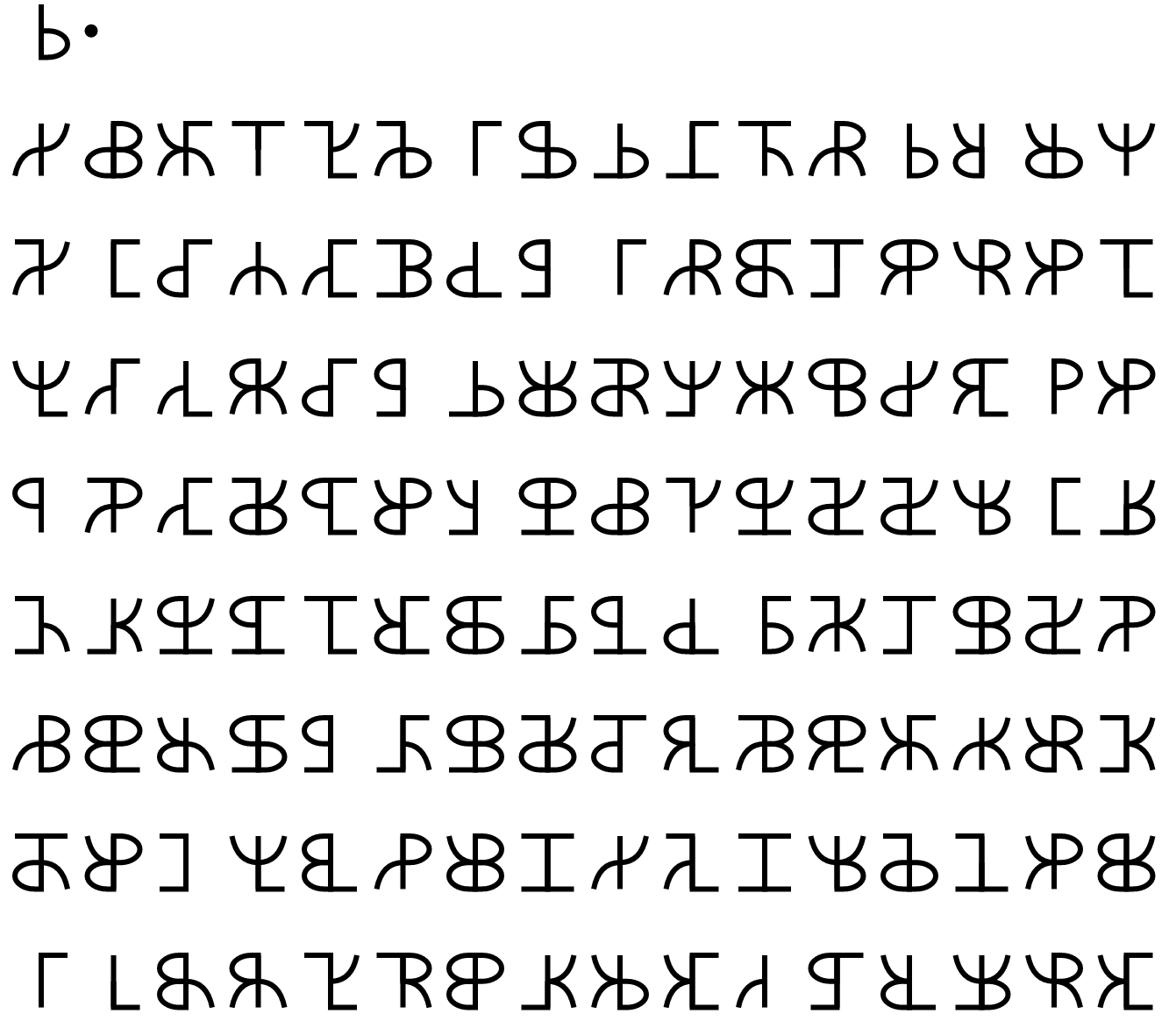
Explanation coming soon, but you may enjoy trying to figure it out on your own.
Here’s something I’ve been playing with:
Explanation coming soon, but you may enjoy trying to figure it out on your own.
Posted in Uncategorized
See previous posts if you’re confused:
Part 1: Normal numbers in base ten
Part 2: Numbers in base φ and π
Part 3: One is normal in base π
This post is also available on LessWrong.
This wasn’t supposed to be a whole series of posts, so we’re going to speed through the punchline:
One is a normal number.
“No it’s not.”
In base π, I mean.
“No, it’s still just 1.“
Don’t be so greedy. Start with 0. and go from there.
“So it’s 0.222… or 0.333… or something?”
Nope, it’s 0.3011021110…
“That’s… bad. Does it repeat?”
I think it’s normal, but that seems hard to prove.
“So each digit occurs equally often?”
No, normal numbers in base π are about a 37%-30%-29%-4% split of 0, 1, 2, 3.
“Where did that distribution come from?”
Integrals of this weird function:
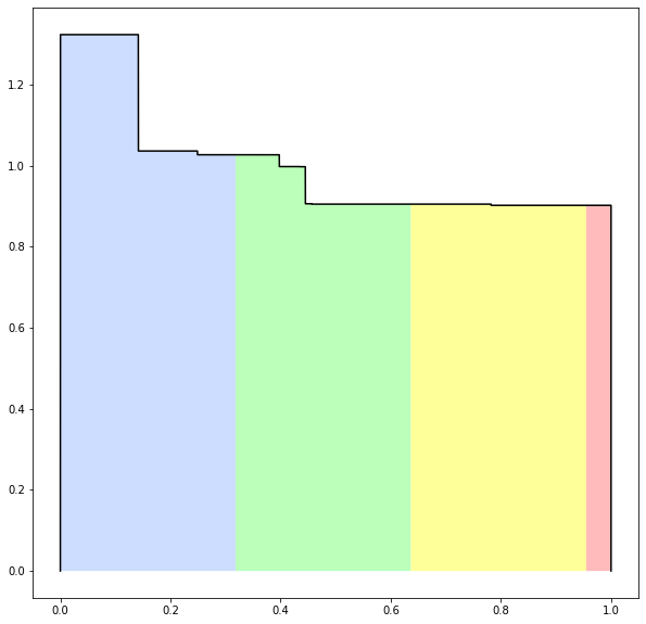
“And where did that come from?”
It’s the distribution of remainders when computing a random number in base π.
“What are the x coordinates of those discontinuities?”
Sequence of remainders when computing 0.3011021110…
“um”
which are dense in [0, 1], by the way.
“Can you prove that?”
No, and neither can you.
“…And the y coordinates?”
The discontinuities get smaller by a factor of π each time.
“And almost all numbers have this distribution of remainders?”
Yup.
“Including 1, if you use the 0.3011021110… representation.”
Yup.
“So the histogram of x-coordinates of the N largest discontinuities in this function approaches… this function itself, as N goes to infinity.”
Yup.
“Which has derivative zero almost everywhere, but has a dense set of discontinuities.”
Yup!
“Any other neat facts about it?”
It’s a fractal.
“How?”
Stretch out the colored regions by a factor of π horizontally, shrink by π vertically, and add them to each other. You get the original function back:
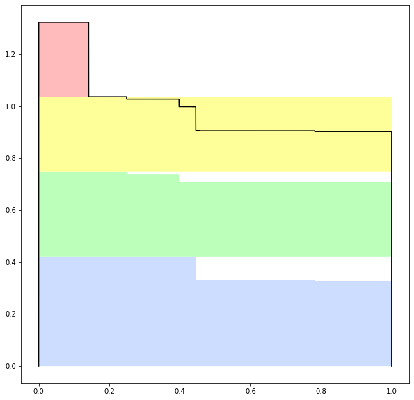
“And this is all because π is normal, or transcendental, or something?”
Nope, I think analogous statements are all true for base 3.5.
Part 1: Normal numbers in base ten
Part 2: Numbers in base φ and π
Part 3: One is normal in base π
(This post assumes familiarity with the concept of number bases: decimal, binary, hexadecimal, and so on.)
Let’s say we want to write numbers in base φ≃1.618_ten (the golden ratio), or base π≃3.14_ten. So, for example, 1000_π = π^3.
The allowed digits are {0, 1} for base φ, and {0, 1, 2, 3} for base π.
Why not just e.g. {0, 1, 2} for π? That wouldn’t be enough digits to express everything: there’s a gap between 0.222…_π = (2π/(π-1) – 2) ≃ 0.934_ten and 1._π = 1._ten.
In integer bases, decimal representations are almost unique (see previously): you can write 5/2 as 2.5_ten or 2.4999…_ten, but that’s the only kind of ambiguity.
In base φ, 100._φ = φ^2 = φ+1 = 11._φ. Uh oh.
Worse still, 110._φ = 1000._φ, which means that 111._φ > 1000._φ. Numbers aren’t lexicographically ordered anymore! Looking at two numbers, it’s not immediately obvious which is bigger.
(But there’s a limit to how bad this gets: the largest number starting with 0. is 0.111…_φ, which is equal to 10._φ. So if two numbers start off with the same digits, and then the first has a 1 where the second has a 0, the second number has to start “catching up” within the next two digit positions or it will end up being smaller.)
Wikipedia has lots of facts about base φ. It describes the “standard form” of a number as the representation that avoids the digit sequence 11, which is always equivalent to the representation given by the greedy algorithm in the previous post. (In short: keep multiplying by the base and chopping off the integer part of the result.)
Mercifully, the greedy/standard representation in any base is unique and sorts lexicographically.
In any base, the greedy algorithm applied to one gives 1.
The second-greediest representation (see previously) in an integer base is always something like 1 = 0.222…_three or 1 = 0.999…_ten.
In base φ, the second-greediest-rep is 1 = 0.11_φ, which terminates.
In base π, it’s 1 = 0.301102111002022113…_π, nonterminating, with no discernable pattern.
(Note that flipping any of the 0s to 1 or 1s to 2 makes the number bigger than one.)
This kind of makes sense — the golden ratio is a much nicer number than pi (algebraic instead of transcendental, etc.).
But in base 5/2, the second-greediest-rep is 1 = 0.2101110000110121…_(5/2), nonterminating, no discernable pattern.
And in base X≃2.732_ten, the positive root of x^2-2x-2, it’s 1 = 0.22_X.
So which numbers have terminating second-greediest-reps for 1?
We can rewrite these representations as expressions like 11._φ = φ^2 and 22._X = X^2. The left-hand sides are polynomials in the base (φ+1 and 2X+2, in these cases), and we end up with the somewhat weird theorem:
The second-greediest-rep for 1 terminates in base B iff B is a root of a monic polynomial whose other coefficients are integers between -floor(B) and 0, inclusive.
What about repeating second-greediest-reps? Integer bases, sure, but any others?
Well, in base φ+1, we get 1 = 0.2111…_(φ+1).
In general, when do we get something repeating?
…Left as exercise for the reader.
As we write down digits for some number in some base B, we can sometimes deviate from the greedy algorithm by writing down something smaller than necessary, leaving a remainder that isn’t in the half-open interval [0, 1).
For the second-greediest representation of a number, we do this once, at the beginning. If the number we’re representing is 1, we have a remainder of 1, which just barely falls outside [0, 1).
But sometimes we can be bolder. How large can the remainder r_i be? Presumably there’s some cap, r_i <= r_max.
Well, the largest contribution we can get from the remaining digits is 0.ddd…_B, where d=ceil(B-1) is the largest digit. And that’s equal to:
r_max = ceil(B-1) / (B-1)
Sanity check: For integer B, this is just 1, and we are only allowed to have remainders in [0, 1]. This is consistent with the fact that tails of 9’s are the only non-greedy representation possible in base ten.
Recall our statements about normal numbers in base ten:
I think the following is true in any base B, and fairly easy to prove:
The sets of numbers for which these two statements are true should be the same; let’s call them “normal numbers”, extending the usual integer-base definition. Furthermore, non-normal numbers may still have “normal representations” (whose remainders follow D(B)) under some non-greedy algorithm.
I think the following is true but probably very difficult to prove:
Note that this is definitely not true in any integer base, or in base phi, where the second-greediest rep of one terminates or repeats.
What does D(π) look like, and what are its properties? See here.
Part 1: Normal numbers in base ten
Part 2: Numbers in base φ and π
Part 3: One is normal in base π
(Warning: This is mostly background information for the other posts.)
Usually, we write numbers in base ten. For example:
π ≃ 3.14159_ten
What is this magic? Let me explain.
First, pick a “base”, which can be any number greater than one. We’ll use ten.
Then, choose “digits”: symbols for some small integers, like 0 for zero and 3 for three.
A decimal representation in base ten is a sequence of these symbols, with a “decimal point” (looks like: .) somewhere.
A symbol just to the left of the decimal point is worth its face value; symbols one position left of that are worth ten times their face value, and symbols one position to the right (just after the decimal point) are worth one tenth of their face value, etc.
Here are some nonobvious but easy-to-prove facts:
“Wait, almost unique?” Yeah, because .99999… (infinite tail of 9s) is equal to 1., and 2.4999… = 2.5, etc. As it turns out, this is the only kind of non-unique representation in base ten. It’s also the only case where lexicographic ordering fails (very slightly: the two representations of these numbers are consecutive lexicographically).
(I’m ignoring leading zeros.)
The nice algorithm is greedy: you insert the most valuable digit you can in every position.
Let’s try to write pi.
First, divide by whatever power of ten you need to make the result less than one. That’s 10^1.
For numbers with two representations (one that is finite, and another ending in a tail of 9s), this algorithm always gives the finite representation.
There are two ways to obtain the string 0.999…:
Here’s a Python snippet for the greedy representation of any number, in any base:
def greedy(base, x, n):
    offset = mp.floor(mp.log(x)/mp.log(base))+1
    x /= mp.power(base, offset)
    dig = []
    rem = []
    r = x
    for _ in range(n):
        rem += [r]
        r *= base
        d = int(r)
        dig += [d]
        r = r - d
    return int(offset), dig, rem
(I’m using mpmath for arbitrary-precision arithmetic.)
You may also find these useful:
def tofloat(offset, base, dig):
    out = 0.
    mult = 1
    for d in dig:
        mult /= base
        out += d * mult
    return out * base**offset

def tostring(offset, dig, rem=None):
    out = ''
    for i, d in enumerate(dig):
        if i == offset:
            out += '.'
        out += (str(d) if d<=9 else f'[{d}]')
    return out
And here’s the “second-greediest representation” in code:
def greedy2(base, x, n):
    offset = mp.floor(mp.log(x)/mp.log(base))+1
    x /= base**offset
    dig = []
    rem = []
    r = x
    rem += [r]
    r *= base
    d = int(r) - 1
    dig += [d]
    r = r - d
    for _ in range(n):
        rem += [r]
        r *= base
        d = int(r)
        dig += [d]
        r = r - d
return int(offset), dig, remMost numbers don’t have a second-greediest representation: if you try to write pi starting with 2., you’ll be in trouble (the largest thing you can end up with is 2.999…, which is three, not pi).
In fact, the following is easy to prove (if you majored in math):
The statement about remainders is equivalent to the statement about substrings, and I think it’s more elegant.
As an example, pi is conjectured (not proven!) to be normal in base ten. Here are histograms of its first thousand digits (3, 1, 4, 1, …), its first thousand digit-pairs (31, 14, 41, 15, …), and two histograms of its first thousand remainders (.1415…, .4159…, .1592…, .5926…, …) with different bin sizes:

As we look at more and more digits of pi, these histograms should each converge to uniform — but nobody has been able to prove it.
We can also define a normal representation as a representation of a number with a uniform limiting distribution of remainders. In base ten, this isn’t very interesting: the only numbers with more than one representation aren’t normal, and neither are either of their representations.
In particular, 1. and 0.999… are definitely not normal.
We’ll need this definition later, though.
New post on the Alignment Forum:
And LessWrong:
Posted in Uncategorized
Here are two bijections between (infinite) bitstrings and (finite or infinite) sequences of positive integers:
You can think of a bitstring as being made up of consecutive runs of one or more 0s or 1s, like “0000” and “111” and “0”.
From bits to integers: Prepend a 0 to the bitstring, then slice it up into runs of 0s and 1s and write down the length of each run. If the string ends in an infinite run, stop the sequence of integers after the last finite run.
From integers to bits: Write down alternating runs of 0s and 1s, with lengths given by the numbers in the sequence. If the sequence stops, write an infinite run of whichever bit value is next. Then delete the first 0.
For example, “001110011100111…” maps to [3, 3, 2, 3, 2, 3…] and “110001100011000…” maps to [1, 2, 3, 2, 3, 2, 3…].
The annoying extra-0 trick is to distinguish pairs of bitstrings like the above, which are flipped versions of each other.
Note that “00000…” maps to [] and “11111…” maps to [1].
On the other hand, you can think of a bitstring as being made up of runs of zero or more 0s ending in a single 1, like “001” and “000001” and “1”.
From bits to integers: For each 1 in the bitstring, write down the number of 0s immediately preceding it plus one. If the bitstring ends in an infinite run of zeros, stop the sequence of integers after the last 1.
From integers to bits: For each number N in the sequence, write down N-1 0s and then one 1. If the sequence stops, write an infinite run of 0s.
Note that “00000…” maps to [] and “11111…” maps to [1, 1, 1, 1, 1…]
The all-zeros string maps to an empty list under both bijections, but the all-ones string is different. It’s also easy to see that these bijections are pretty different on a generic bitstring.
Suppose we start with the list [1] and repeatedly do the following:
What does the sequence of bitstrings look like?
The first few steps look like this:
[1] –> 11111…
11111… –> [1, 1, 1, 1, 1…]
[1, 1, 1, 1, 1…] –> 101010…
101010… –> [1, 2, 2, 2…]
[1, 2, 2, 2…] –> 110011…
So our first few bitstrings are:
11111111…
10101010…
11001100…
I’ll let you discover the pattern for yourself (pen and paper is sufficient, but Python is faster), but if you get impatient CLICK HERE to see the first 64 bits of each of the first 64 strings.
This is a somewhat technical / context-heavy AI alignment post:
https://www.alignmentforum.org/posts/A9eAPjpFjPwNW2rku/gradient-hacking-via-schelling-goals
There are some comments on the mirrored post on LessWrong:
https://www.lesswrong.com/posts/A9eAPjpFjPwNW2rku/gradient-hacking-via-schelling-goals
Suppose you have a binary classifier. It looks at things and tries to guess whether they’re Dogs or Not Dogs.
More precisely, the classifier outputs a numeric score, which is higher for things it thinks are more likely to be Dogs.
There are a bunch of ways to assess how good the classifier is. Many of them, like false-positive rate and false-negative rate, start by forcing your classifier to output discrete predictions instead of scores:
A lot of metrics — like F1 score — also assume a population with a particular ratio of Dogs to Not Dogs, which can be problematic in some applications.
The AUC metric doesn’t require a fixed threshold. Instead, it works as follows:
Or rather, that’s one way to define it. The other way is to draw the ROC curve, which plots the relationship between true-positive rate (sensitivity) and false-positive rate (1-specificity) as the classification threshold is varied. AUC is the Area Under this Curve. That means it’s also the average sensitivity (averaged across every possible specificity), and the average specificity (averaged across sensitivities). If this is confusing, google [ROC AUC] for lots of explanations with more detail and nice pictures.
AUC is nice because of the threshold-independence, and because it’s invariant under strictly-monotonic rescaling of the classifier score. It also tells you about (an average of) the classifier’s performance in different threshold regimes.
Sometimes, though, you care more about some regimes than others. For example, maybe you’re okay with misclassifying 25% of Not Dogs as Dogs, but if you classify even 1% of Dogs as Not Dogs then it’s a total disaster. Equivalently, suppose you care more about low thresholds for Dogness score, or the high-sensitivity / low-specificity corner of the ROC curve.
As I recently figured out, you can generalize AUC to this case! Let’s call it N-AUC.
There are two ways to define N-AUC, just as with AUC. First way:
Second way:
Fun exercise: These are equivalent.
Of course, 1-AUC is just the usual AUC.
You can also emphasize the opposite high-threshold regime by comparing one Dog to N Not Dogs, or integrating (specificity)^(N-1).
In fact, you can generalize further, to (N,M)-AUC:
Compute P(N Dogs > M Not Dogs), or integrate (sensitivity)^(N-1) * (specificity)^(M-1) under the curve. For large, comparable values of M and N, this weights towards the middle of the ROC curve, favoring classifiers that do well in that regime.
I thought of this generalization while working on Redwood’s adversarial training project, which involves creating a classifier with very low false-negative rate and moderate false-positive rate. In that context, “Dogs” are snippets of text that describe somebody being injured, and “Not Dogs” are snippets that don’t. We’re happy to discard quite a lot of innocuous text as long as we can catch nearly every injury in the process. Regular old AUC turned out to be good enough for our purposes, so we haven’t tried this version, but I thought it was interesting enough to make for a good blog post.
A friend pointed me to a fun puzzle. There’s a fairly-straightforward “standard” solution, but I had some extra fun finding increasingly weird ones.
This post is really about abstract algebra, but I’m going to try to keep the prerequisites low by spelling everything out. Target audience: people who like abstract algebra, mathy puzzles, or both.
Here’s the puzzle: https://www.futilitycloset.com/2021/08/27/50-for-all/
A puzzle by Ben H., a systems engineer at the National Security Agency, from the agency’s August 2016 Puzzle Periodical:
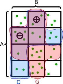
At a work picnic, Todd announces a challenge to his coworkers. Bruce and Ava are selected to play first. Todd places $100 on a table and explains the game. Bruce and Ava will each draw a random card from a standard 52-card deck. Each will hold that card to his/her forehead for the other person to see, but neither can see his/her own card. The players may not communicate in any way. Bruce and Ava will each write down a guess for the color of his/her own card, i.e. red or black. If either one of them guesses correctly, they both win $50. If they are both incorrect, they lose. He gives Bruce and Ava five minutes to devise a strategy beforehand by which they can guarantee that they each walk away with the $50.
Bruce and Ava complete their game and Todd announces the second level of the game. He places $200 on the table. He tells four of his coworkers — Emily, Charles, Doug and Fran — that they will play the same game, except this time guessing the suit of their own card, i.e. clubs, hearts, diamonds or spades. Again, Todd has the four players draw cards and place them on their foreheads so that each player can see the other three players’ cards, but not his/her own. Each player writes down a guess for the suit of his/her own card. If at least one of them guesses correctly, they each win $50. There is no communication while the game is in progress, but they have five minutes to devise a strategy beforehand by which they can be guaranteed to walk away with $50 each.
For each level of play — 2 players or 4 players — how can the players ensure that someone in the group always guesses correctly?
I strongly encourage you to solve this puzzle yourself before reading on. I was tempted to read the answer, but had more fun figuring it out (I went down a blind alley at first).
We can generalize this puzzle to the case with N different “colors” or “suits” of cards and N players.
Here’s the standard solution: (For a less mathy version, see the Futility Closet link.)
More generally, suppose we have a function W from N card suits to a number mod N.
(The standard solution (for N=4) is to let W(a, b, c, d) = (a + b + c + d) % 4, where “%” is the mod operator.)
Each player guesses a different value for W. For example, taking N=4 again, the third player always guesses that W=2. In order for the strategy to work, the equation W(a, b, c, d) = 2 needs to have a unique solution for c in terms of a, b, d. (And similarly, W(a, b, c, d) = 0 needs to be solvable for a, and so forth.)
This is easy to verify for the standard solution, but it’s not immediately obvious how to construct other functions with this property.
What if we want a different strategy? Well, to start with, we can give the players different numbers — maybe Doug is 3 and Fran is 2 instead of vice-versa. Or we can give the suits different numbers. (If we do both, some combinations of choices will give the same strategy, though.)
There are some easy and dumb ways to go further. For one thing, the assignment of numbers to suits can be different depending on whose card it is (but not depending on who’s looking at it!).
Tricks like this give a pretty large number of essentially-the-same solutions, which I’m not really interested in counting.
Addition mod N is a way to “add up” a bunch of numbers in the set {0, 1, …, N-1} and also lets you subtract them. There are other ways to do this: an example for N=4 is to write numbers in binary, {00, 01, 10, 11}, and separately add the bits mod 2. (You can think of this as bitwise-XORing the numbers if you like to code in C.)
So there’s another solution: W(a, b, c, d) = a XOR b XOR c XOR d.
(Exercise: Show that this works if and only if N is a power of 2.)
What can we do for arbitrary N?
Well, we can generalize the two-bit strategy: if N = X * Y, we can map our N numbers to pairs (x, y), where 0 <= x < X and 0 <= y < Y. Then we can add two pairs by adding their parts separately, mod X and mod Y respectively. And we can get recursive, by breaking down X = Z * W….
In general, any way of adding and subtracting things — such that the order you do it in doesn’t matter — is an abelian group. (I’m hiding some axioms in the words “adding and subtracting”. For example, adding something and then subtracting it shouldn’t do anything.)
There’s a cute theorem that says that any finite abelian group is of the form above: it’s a direct sum of cyclic groups. (A “cyclic group” is addition mod N for some N, and a “direct sum” is the pairing construction above. Confusingly, “direct product” and “direct sum” mean the same thing in this context.)
So we’re done, right?

Not all groups are abelian — sometimes the order matters. Also, not all groups are groups of numbers; sometimes they’re groups of other things.
Here’s a cute example: take the N=24 case. Instead of numbers from 0 to 23, assign each player a different way to permute four things. For example, maybe Doug is assigned “swap the first two things and leave the other two in place”. There are 4! = 24 ways to permute four things, so this works. Also, assign each suit a different 4-permutation as well.
Now, when you go to “add up” some suit and player permutations, do it by setting out four objects, applying each permutation one after another, and then seeing what overall permutation you end up with. In other words, W(a, b, c, d) = a∘b∘c∘d, where (a, b, c, d) are four permutations and “x∘y” represents composition of permutations (doing x and then doing y).
This time, it matters what order you do it in (e.g. whether you do Doug’s permutation before or after Fran’s). (Exercise: Find two permutations that don’t commute: a∘b ≠ b∘a.)
The strategy is still the same: “adding up” everyone else’s cards and “subtracting” that from your own number. The only difference is that it’s kind of annoying to work out the order to do that in, and the subtraction has to happen somewhere in the middle sometimes. (Exercise: Fill in the details here, and explain what “subtracting” a permutation means.)
In addition to modular arithmetic and permutation groups, there are tons of other places groups show up — symmetries of geometric objects are one of my favorites. This post is already too long, so I’ll save the group propaganda for the future.
Is there a cute theorem that tells you what all the possible finite groups are?
No, there’s a fairly messy theorem with an enormous proof. It took hundreds (thousands?) of mathematician-years to prove it, and the result was so long (sprawling across countless papers in math journals) that a few brave souls have been working on a condensed “second-generation” version. The first volume of the second-generation proof was published in 1994; the ninth volume came out this year. There will probably be four more volumes. The group classification megaproject is an incredible achievement, and one of the worst theorems I’ve ever heard of.
Worse yet, it only classifies the finite simple groups. I won’t define “simple” here, but the upshot is:
So it’s not really clear, philosophically, that what I’ve given you in this section is a “solution” to the puzzle at all. What I’ve given you is a machine for turning finite groups into solutions. You also need some feedstock for the machine: here‘s all the groups for N<32.
But there’s no known systematic way to find all the groups of order N, for arbitrary N. We don’t even know how many groups of order 2048 there are.

Here’s another thing you can do: add up the four suits (a, b, c, d) as follows:
W(a, b, c, d) = (a ∘ b) + (c # d)
…where ∘, +, and # are the group operations for three different groups.
So, for example, you can add the first two and last two numbers mod 4, then convert the sums to binary and add them (mod 2, mod 2).
(Exercise: Show that this is still a puzzle solution (i.e. you can still solve for a, b, c, or d.))
When you need to “translate” between groups (e.g. turn a permutation-of-n-things into a number-mod-n!), you can do it totally arbitrarily! Just make sure the translation you use is a one-to-one mapping. (Exercise: show that this is okay.)
This gives a huge explosion of strategies. Also, now the overall operation isn’t even associative, so you have to be careful and not do W = a ∘ ((b + c) # d) by mistake — that’s a totally different solution.

Fun fact: despite all the terrible solutions above, none of them give interestingly-different answers to the cases where N is prime, such as N=2, 3, or 5. The only variety for those cases comes from the relabeling tricks: assigning different card-number mappings per player, and “translating” intermediate values in the computation via arbitrary permutations. That’s because the only groups of prime order are cyclic groups, which give you the standard solution to the puzzle.
It’s time to rectify that. (There’s a pun here somewhere — “rectify”, Latin, rectus, square, rectangle… oh well.)
Groups have to be associative, so that (a∘b)∘c = a∘(b∘c). As we just saw, solutions to this puzzle don’t need to be associative, so there’s no need to limit ourselves to binary operations that come from groups.
There’s two perspectives here:
(1): A group without the requirement of associativity is a quasigroup. Group theory is a beautiful subject; quasigroup theory is an ugly one.
(2): The multiplication table of a quasigroup is a Latin square, which is basically a solved Sudoku without the smaller 3×3 boxes.

There’s no hope of enumerating these quickly or easily. By relaxing the amount of structure of our solutions too far, we have passed beyond the event horizon of classifiability. There is no theorem for these, nice or otherwise. They have some cool connections, though, like the design of statistical experiments. And they look nice in stained glass.
For a binary operator, the multiplication table is a square. But there’s no need to restrict ourselves to combinations of binary operators.
A Latin cube (or hypercube) is like a Latin square, but in more dimensions.
With three Latin squares X, Y, Z, we can write equations like
W(a, b, c, d) = X[Y[a, b], Z[c, d]],
where X[i, j] is the entry in the i-th row and j-th column of X. This should look pretty familiar; it’s the same as the expression (a Y b) X (c Z d) for the corresponding quasigroup operations X, Y, Z.
With a Latin cube C and a square S, we instead have things like
W(a, b, c, d) = C[a, S[b, c], d]
You could interpret the Latin cube as the multiplication table for a ternary operator in some sort of awful algebraic structure, but why make life hard for yourself?
A Latin N-cube is almost the last word on solutions to this puzzle, since it’s equivalent to a function W such that
W(a, b, c….) = w
can be solved uniquely for a, or b, or c, etc.
But this is slightly stronger than what we asked for, which was:
In order for the strategy to work, the equation W(a, b, c, d) = 2 needs to have a unique solution for c in terms of a, b, d. (And similarly, W(a, b, c, d) = 0 needs to be solvable for a, and so forth.)
We only need the equation to be solvable for the w-th argument (counting from zero).
But are there any solutions like this that aren’t full Latin hypercubes?
Yup. It’s not too hard to find one with a backtracking search; I did N=3 by hand in a few minutes.
Any solution to the puzzle has to be of this form.
(Exercise: Show that every solution has exactly one winner, no matter what the suits are. W specifies this winner in terms of those suits. Show that every strategy is equivalent to “assume the winner is going to be you, then solve the equation W(a, b, c…) = You to find your suit”.)
But by the same token, this form is not very helpful; a “generalized Latin hypercube” W is just an arbitrary array of N^N values, with the constraint that it must solve this puzzle.
The solutions in this post are on a spectrum, with the standard solution being the simplest and easiest to execute, and later solutions being increasingly weird and also increasingly hard to construct explicitly. I think the most interesting ones are probably the non-abelian groups, since they have the most fun math involved (pick your favorite Platonic solid; its group of symmetries specifies a puzzle solution for 24, 48, or 120 players) but your mileage may vary.
It’s kind of like this:

On the left, the standard solution. In the middle, group solutions. On the right, Latin hypercube solutions.
Ponder this mystery.
Exciting news today: the kilogram is officially going to be redefined. More specifically, it’s being redefined “based on physical constants”. Also, all the other SI units are being redefined “based on physical constants” at the same time.
“Wait, how does that work? If they’re all being redefined, what’s special about the kilogram? What’s the current definition? Who’s in charge of that anyway?”
Last things first: the BIPM (Bureau International des Poids et Mesures, International Bureau of Weights and Measures) has been in charge of these things since May 20, 1875. Delegates from the member states of the BIPM meet, roughly every four years, at the CGPM (Conférence générale des poids et mesures, General Conference on Weights and Measures), and the 26th CGPM just voted to adopt the new definitions next year, on May 20 (date chosen for symbolic reasons, or so I assume).
I think it’s easiest to understand the “New SI” as encompassing two principles.
The first principle, which I’ll call “universality”, is that units should be based on objects for which perfectly identical copies are already universally available — like atoms or molecules, and unlike metersticks or the planet Earth. This requires a lot of practical changes to how units are defined and measured. It’s an idea that’s been gaining ground for centuries: James Clerk Maxwell said in 1870 that “If…we wish to obtain standards of length, time and mass which shall be absolutely permanent, we must seek them not in the dimensions, or the motion, or the mass of our planet, but in the wavelength, the period of vibration, and the absolute mass of these imperishable and unalterable and perfectly similar molecules.” (Quote borrowed from PhysicsWorld.)
The current definitions of the meter and second are compliant with this principle; the kilogram isn’t, but that’s about to change.
The second principle is that units should be defined by reference to the values of physical constants, not by reference to physical measurements. This is a bit subtler, and also — I’m going to argue — purely semantic. If you do the legwork of following the first principle, you tend to end up at the second one, whereas the second principle doesn’t function very well on its own (but can be adopted whenever you like by changing the language you use).
All of the SI units are being “redefined” in May in accordance with the second principle. This doesn’t change anything in practice, but it’s sort of aesthetically appealing, so there’s that.
That’s enough metrological philosophizing. Let’s learn some history.
The SI is the International System of Units, aka the “metric system”. It’s used directly by most of the world’s population, and used indirectly even in the US; the foot is officially defined as 0.3048 meters.
Back in the ancient past (before 1960), the meter was defined as the length of a meterstick. More precisely, a particular platinum-iridium meterstick (the International Prototype Metre) kept at the BIPM.
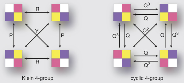
From 1960 to 1983, the meter was defined (per Wikipedia) as “1 650 763.73 wavelengths of the orange-red emission line in the electromagnetic spectrum of the krypton-86 atom in a vacuum”. We can choose to view this in two ways: either we’re measuring a bunch of wavelengths of some light (from a specific source) and calling that our meterstick, or we’re fixing a particular physical constant, the wavelength of the orange-red emission line of Kr-86, to be equal to (1/1 650 763.73) meters exactly. The 1960 definition clearly satisfies the first principle I mentioned — the definition is based on something universally replicable — but it fails the second principle, entirely because an artifact-based phrasing was chosen instead of a constant-based one.
This is what krypton’s spectrum looks like. The orange line is the one we’re talking about. Source: Adric Riedel
These days (since 1983) the meter is defined as the length of the path travelled by light in vacuum during a time interval of 1/299 792 458 of a second. This again follows the first principle (universality) and still technically fails the second: the distance traveled in some interval isn’t quite a physical object, but it’s a particular thing one meter in length that you can visualize.
This is being replaced in May by a new definition which uses the fixing-a-constant language: The meter will be defined by taking the fixed numerical value of the speed of light in vacuum, c, to be 299 792 458 m/s.
If you wanted to, you could even rewrite the meterstick-based definition in terms of a “constant”: before 1960, the meter was defined by the requirement that the physical constant known as “the length of the International Prototype Metre” have the value “1 meter”.
You might object that this isn’t really a universal physical constant — there’s only one International Prototype Metre, but there’s identical copies of the Kr-86 atom (and its emitted light) everywhere in the universe. This shows that the second principle (constant-oriented phrasing) is at best unappealing without the first one (universality): if we’re basing our unit on a complex, unique objects like the Prototype Metre, which can get damaged or lost or just gradually change its shape, then the “constants” involved won’t be very interesting ones.
The second, by the way, is defined as 9 192 631 770 periods of the hyperfine transition of cesium. The term “hyperfine transition” requires a lecture on quantum physics, but I’ll try to summarize.
Imagine two magnets. If you place them next to each other with the north poles facing the same direction, they’ll try to squirm out of your grasp. As long as you hold them in place, there’s potential energy which is just waiting to become kinetic energy (e.g. by flinging one magnet across the room). If you flip one magnet around, the magnets will cling to each other quietly. There’s less potential energy. (In fact, negative potential energy: you need to apply some force to separate them.)
Cesium atoms are like that, but one magnet is the nucleus and the other is the electron cloud. (It’s like a really tiny electromagnet: a loop of electric current (the electrons in their orbits) generates a magnetic field.) There’s an unstable high-energy state with the nucleus and electrons pointing the same way, and a stable low-energy state where they’re pointing in opposite directions.
Here’s a diagram of the hyperfine transition, on a plaque that we strapped to the Pioneer spacecraft and flung into interstellar space. Hopefully, aliens will be able to figure out what it means, so that we can establish a common system of units with them. Source: ScienceCavern
If the cesium atom is in the high-energy state, it will rearrange itself into the low-energy state, ditching the (very tiny) excess energy by emitting a (very low-energy) photon. That photon will have a frequency of 9 192 631 770 Hz, ie, it oscillates 9 192 631 770 times every second. This is related to the energy difference by E = h ν, where h is Planck’s constant and ν (nu) is the frequency.
While we’re at it, the wavelength λ (lambda) of that photon is given by λ = c/ν, where c is the speed of light. This works out to (299 792 458/9 192 631 770) meters, or about an inch and a quarter. So if you aren’t convinced yet that the current definition of the meter can really be considered “artifact-based”, here’s an equivalent definition that’s very similar to the old krypton-89 one:
One meter is the length of (9 192 631 770/299 792 458) wavelengths of the light emitted when the little magnets inside cesium flip into proper alignment.
Right now, the kilogram is a bit of an embarrassment. It’s defined as the mass of the International Prototype Kilogram, a platinum-iridium cylinder that lives at the BIPM, thereby failing the universality principle. But that’s about to change!
Starting next year (per today’s BIPM resolution), the kilogram will be defined by requiring Planck’s constant, h, to have the value 6.62607015×10⁻³⁴ kg m2/s.
This is a constant-based definition, to match the constant-based definitions that are being adopted at the same time for the second, meter, etc. But as I’ve argued, the difference between fixing a constant and measuring a physical artifact is more or less semantic. The really important thing is that we’re picking a better artifact. So it’s interesting to ask what definition we’d be using next year if the BIPM had decided to square away the universality issue before worrying about basing things on constants.
In other words, if you interpret the new kilogram as the mass of some reference object, what object would that be?
Well, the most famous equation in physics tells us that E equals m c squared. Or, as Einstein originally wrote it, m = E/c2. (No, really.) What this means is that the presence of energy in an object always contributes a little bit (a tiny bit!) to the object’s mass. In fact, according to Einstein, that’s all mass is: internal energy by a different name. Does this mean that cesium is slightly heavier when it’s in the higher-energy state? Yup!
By how much? Combining m = E/c2 and E = h ν, we find that it’s m = h ν/c2.
Dividing “1 kg” by that expression, we find that the new definition of the kilogram is exactly equivalent to this one:
One kilogram is the extra mass present in (299 792 458)2/(6.62607015×10−34 × 9 192 631 770) cesium atoms if they’re all in the excited hyperfine state (magnets pointing the same way) instead of the ground state (magnets pointing in opposite directions).
However, I don’t recommend you try to make that measurement directly; you’d need a few trillion tons of cesium, and as soon as it all decays to the ground state, you’ll be bombarded with a kilogram’s worth of energy. (It’s enough energy to power San Francisco for a couple of years.)
But in principle, a kilogram can still be thought of as the mass of a specific defining thing. Just not a thing that can get lost or damaged, or gradually lose mass over time.
Posted in Uncategorized

